Not my original post. However made some updates minor in the posts with latest version
Freeze Tensorflow models and serve on web
So you trained a new model using Tensorflow and now you want to
show it off to your friends and colleagues on a website for a hackathon
or a new startup idea. Let’s see how to achieve that.
1. What is Freezing Tensorflow models?
Neural
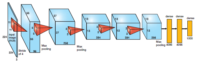
networks are computationally very expensive. Let’s look at the
architecture of alexnet which is relatively simple neural network:
Let’s calculate the number of variables required for prediction:
conv1 layer: (11*11)*3*96 (weights) + 96 (biases) = 34944
conv2 layer: (5*5)*96*256 (weights)+ 256 (biases) = 614656
conv3 layer: (3*3)*256*384 (weights) + 384 (biases) = 885120
conv4 layer: (3*3)*384*384 (weights) + 384 (biases) = 1327488
conv5 layer: (3*3)*384*256 (weights) + 256 (biases) = 884992
fc1 layer: (6*6)*256*4096 (weights) + 4096 (biases) = 37752832
fc2 layer: 4096*4096 (weights) + 4096 (biases) = 16781312
fc3 layer: 4096*1000 (weights) + 1000 (biases) = 4097000
This is more than 60 million parameters that we shall need to calculate a prediction on one image. Apart
from it, we also have similar number of gradients that are calculated
and used to perform backward propagation during training.
Tensorflow models contain all of these variables. Think about it, you
don’t need the gradients when you deploy your model on a webserver so
why carry all this load. Freezing is the process to identify and save
all of required things(graph, weights etc) in a single file that you can
easily use.
- model-ckpt.meta: This contains the complete graph. [This
contains a serialized MetaGraphDef protocol buffer. It contains the
graphDef that describes the data-flow, annotations for variables, input
pipelines and other relevant information]
- model-ckpt.data-0000-of-00001: This contains all the values of variables(weights, biases, placeholders,gradients, hyper-parameters etc).
- model-ckpt.index: metadata. [
It’s an immutable table(tensoflow::table::Table). Each key is a name of
a Tensor and it’s value is a serialized BundleEntryProto. Each
BundleEntryProto describes the metadata of a Tensor]
- checkpoint: All checkpoint information
So,
in summary, when we are deploying to webserver we want to get rid of
unnecessary meta-data, gradients and unnecessary training variabels and
encapsulate it all in a single file . This single encapsulated file(.pb
extension) is called “frozen graph def”. It’s essentially a serialized graph_def protocol buffer written to disk.
In the next section, we shall learn how we can freeze the trained model.
2. Freezing the graph:
We
have a trained model and we want to selectively choose and save the
variables we will need for inference. You can download the model from here. Here are the steps to do this:
- Restore the model (load graph using .meta file and restore weights inside a session). Convert the graph to graph_def.
|
|
saver = tf.train.import_meta_graph('./dogs-cats-model.meta', clear_devices=True)
graph = tf.get_default_graph()
input_graph_def = graph.as_graph_def()
sess = tf.Session()
saver.restore(sess, "./dogs-cats-model")
|
- We choose which outputs we want
from the network. A lot of times you will only be choosing the
prediction node. But it’s possible to choose multiple values so that
multiple graphs are saved. In our case, we want only y_pred as we want
the predictions.
- Now,
we shall use convert_variables_to_constants function in graph_util to
pass the session, graph_def and the ends that we want to save.
|
|
output_node_names="y_pred"
output_graph_def = graph_util.convert_variables_to_constants(
sess, # The session
input_graph_def, # input_graph_def is useful for retrieving the nodes
output_node_names.split(",")
)
|
- Finally we serialize and write the output graph to the file system.
|
|
output_graph="/dogs-cats-model.pb"
with tf.gfile.GFile(output_graph, "wb") as f:
f.write(output_graph_def.SerializeToString())
sess.close()
|
Look at the size of the model. This has reduced significantly from 25 MB to 8.2 MB.
3. Using the frozen Model:
Now, let’s see how we shall use this frozen model for prediction.
Step-1: Load the frozen file and parse it to get the unserialized graph_def
|
|
frozen_graph="./dogs-cats-model.pb"
with tf.gfile.GFile(frozen_graph, "rb") as f:
restored_graph_def = tf.GraphDef()
restored_graph_def.ParseFromString(f.read())
|
Step-2: Now, we just import the graph_def using tf.import_graph_def function.
|
|
with tf.Graph().as_default() as graph:
tf.import_graph_def(
restored_graph_def,
input_map=None,
return_elements=None,
name=""
)
|
This function takes a few parameters:
input_map: A dictionary mapping input names in restored_graph_def to Tensors
return_elements:
You can choose to return specify Tensors/Operations from
import_graph_def. The name of the operations can be specified in
return_elements like this.
|
|
a, b= tf.import_graph_def(graph_def,
return_elements=['inputs',
'fc8/predictions'],
name='')
|
Now,
the complete graph with values has been restored and we can use this to
predict like we earlier did. Here is the complete code.
1
2
3
4
5
6
7
8
9
10
11
12
13
14
15
16
17
18
19
20
21
22
23
24
25
26
27
28
29
30
31
32
33
34
35
36
37
38
39
40
41
42
43
44
45
46
47
48
49
|
import tensorflow as tf
import os
import numpy as np
import os,glob,cv2
import sys,argparse
# First, pass the path of the image
dir_path = os.path.dirname(os.path.realpath(file))
image_path=sys.argv[1]
filename = dir_path +'/' +image_path
image_size=128
num_channels=3
images = []
## Reading the image using OpenCV
image = cv2.imread(filename)
## Resizing the image to our desired size and preprocessing will be done exactly as done during training
image = cv2.resize(image, (image_size, image_size), cv2.INTER_LINEAR)
images.append(image)
images = np.array(images, dtype=np.uint8)
images = images.astype('float32')
images = np.multiply(images, 1.0/255.0)
## The input to the network is of shape [None image_size image_size num_channels].
## Hence we reshape.
x_batch = images.reshape(1, image_size,image_size,num_channels)
frozen_graph="./dogs-cats-model.pb"
with tf.gfile.GFile(frozen_graph, "rb") as f:
graph_def = tf.GraphDef()
graph_def.ParseFromString(f.read())
with tf.Graph().as_default() as graph:
tf.import_graph_def(graph_def,
input_map=None,
return_elements=None,
name=""
)
## NOW the complete graph with values has been restored
y_pred = graph.get_tensor_by_name("y_pred:0")
## Let's feed the images to the input placeholders
x= graph.get_tensor_by_name("x:0")
y_test_images = np.zeros((1, 2))
sess= tf.Session(graph=graph)
### Creating the feed_dict that is required to be fed to calculate y_pred
feed_dict_testing = {x: x_batch}
result=sess.run(y_pred, feed_dict=feed_dict_testing)
print(result)
|
4. Deploying to a webserver:
Finally,
we shall deploy this model to a python webserver. We will install
python webserver and deploy the code. The webserver will allow user to
upload an image and then will generate a prediction i.e. if it’s a dog
or cat. Let’s start with installing flask webserver. Here is how you can
install flask.
Now, we shall add all the code we discussed above in a webapp.py file
after creating a flask app. Let’s first create a flask app:
|
|
import flask
app = flask.Flask(__name__)
|
The frozen weights are 8 MB in our case. If webserver has to load
weights for each request and then do the inference, it will take a lot
more time. So, we shall create the graph and load the weights and keep
that in the memory so that we can quickly serve each incoming request.
1
2
3
4
5
6
7
8
9
10
11
12
13
14
|
def load_graph(trained_model):
with tf.gfile.GFile(trained_model, "rb") as f:
graph_def = tf.GraphDef()
graph_def.ParseFromString(f.read())
with tf.Graph().as_default() as graph:
tf.import_graph_def(
graph_def,
input_map=None,
return_elements=None,
name=""
)
return graph
|
And then call this function at the start of the webserver, so that it’s accessible for each request and happens only once.
|
|
app.graph=load_graph('./dogs-cats-model.pb')
if __name__ == '__main__':
app.run(host="0.0.0.0", port=int("5000"), debug=True, use_reloader=False)
|
Finally, we create an end-point for our web-server which allows an user to upload an image and run prediction:
1
2
3
4
5
6
7
8
9
10
11
12
13
14
15
16
17
18
19
20
21
22
23
24
25
26
27
28
29
30
31
32
33
34
35
36
37
38
39
40
|
@app.route('/demo',methods=['POST','GET'])
def demo():
if request.method == 'POST':
//Code for prediction/inference goes here
return '''
<!doctype html>
<html lang="en">
<head>
<title>Running my first AI Demo</title>
</head>
<body>
<div class="site-wrapper">
<div class="cover-container">
<nav id="main">
<a href="http://localhost:5000/demo" >HOME</a>
</nav>
<div class="inner cover">
</div>
<div class="mastfoot">
<hr />
<div class="container">
<div style="margin-top:5%">
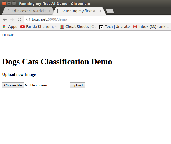
<h1 style="color:black">Dogs Cats Classification Demo</h1>
<h4 style="color:black">Upload new Image </h4>
<form method=post enctype=multipart/form-data>
<p><input type=file name=file>
<input type=submit style="color:black;" value=Upload>
</form>
</div>
</div>
</div>
</div>
</div>
</body>
</html>
'''
|
Once, done we can upload an image using the UI here:
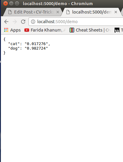
After clicking, upload you can see the results like this:
Hopefully, this post helps you in showing off your newly trained
model. May be you could build the hotDog vs not-hotDog model and raise
millions of dollars for your cool new startup. However, the way to
deploy a tensorflow model on production is Tensorflow-Serving
infrastructure which we shall cover in a future post. The code shared in
this post can be downloaded from our
github repo.


Comments
Post a Comment